Differential Expression Analysis with DESeq2
Introduction
This tool performs differential expression analysis of count data generated from RNA-seq experiments. Based on the DESeq2 program, it enables the identification of differentially expressed genomic features (e.g., genes) through comparisons between experimental conditions.
The software package DESeq2, part of the Bioconductor project, models count data using a negative binomial distribution. It estimates gene-wise dispersion and fold changes, and applies statistical tests to determine whether observed differences in expression between conditions are statistically significant.
Please cite DESeq2 as: Love MI, Huber W, Anders S (2014). Moderated estimation of fold change and dispersion for RNA-seq data with DESeq2. Genome Biology, 15, 550. https://doi.org/10.1186/s13059-014-0550-8
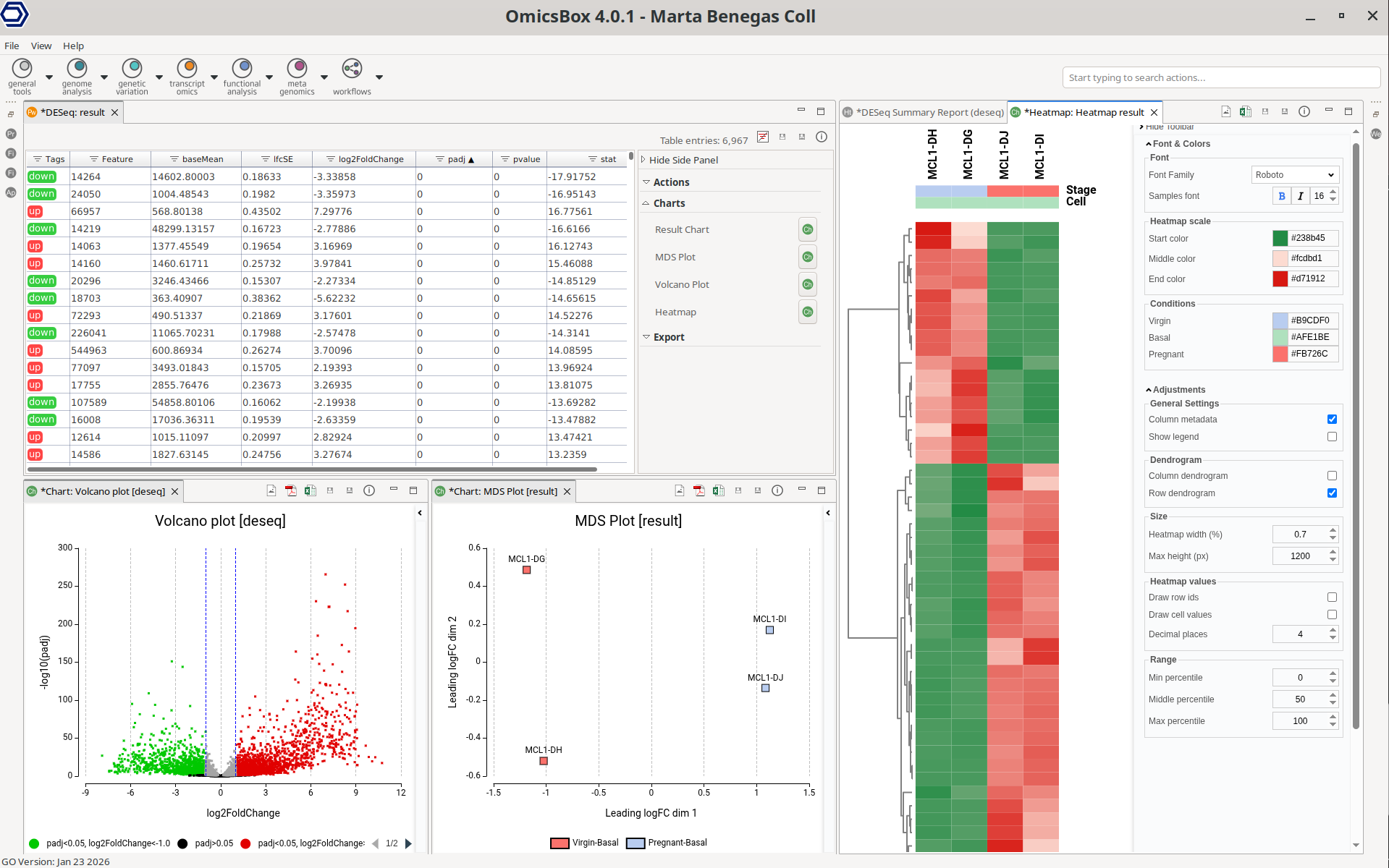
Figure 1: Differential Expression Analysis Interface
Expression Data
The pairwise differential expression analysis application expects gene expression levels in the form of a count table. In OmicsBox, count tables can be generated via the Create Count Table application.
Count tables can also be imported from a text file. Go to transcriptomics → Load → Load RNA-Seq Count Table (expression data) (Figure 2) and select your .txt file containing the count table.
Notes:
- This application only accepts raw counts without any type of normalization.
- Replicates for each experimental condition are necessary.
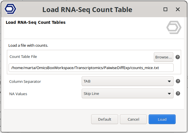
Figure 2: Load Count Table from File
Run Pairwise Differential Expression Analysis
Go to transcriptomics → Differential Expression Analysis. If there’s no count table project opened, the first wizard page (Figure 3) will ask to upload either a Count Table Project (.box file) or a Count Table File (.txt, .csv, or .tsv file). On the second wizard page, choose the "Pairwise Differential Analysis with DESeq2" option.
If a count table is already loaded in OmicsBox (see above section), this one will be used to perform the analysis. You can run the analysis either in transcriptomics → Differential Expression Analysis or via the Side Panel → Actions → Differential Expression Analysis. In this case, the first wizard page will be to select the type of differential expression analysis (Figure 4). In the next pages, it is possible to specify different analysis parameters.
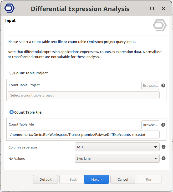
Figure 3: Input wizard page.
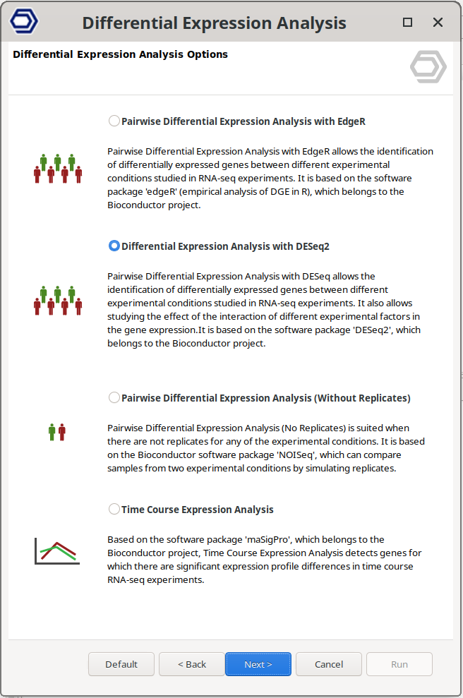
Figure 4: Differential Expression Analysis Options wizard page.
Experimental Design Page
- Experimental design file: Select a .txt file containing experimental factors with the experimental conditions associated with each sample in tab-delimited format. As shown below, rows correspond to samples and columns to experimental factors. Make sure that the names in the first column of the experimental design table are exactly the same as the sample names in the count table header. If your experimental design file has fewer samples than in the count table, only the samples contained in this file will be analyzed.
Name    Strain
SRR3666079  FA1090
SRR3666080  FA1090cpxA
SRR3666081  FA1090cpxR
SRR3666082  FA1090
SRR3666083  FA1090cpxA
SRR3666084  FA1090cpxR
SRR3666085  FA1090
SRR3666086  FA1090cpxA
SRR3666087  FA1090cpxR
SRR3666088  FA1090
SRR3666089  FA1090cpxA
SRR3666090  FA1090cpxR
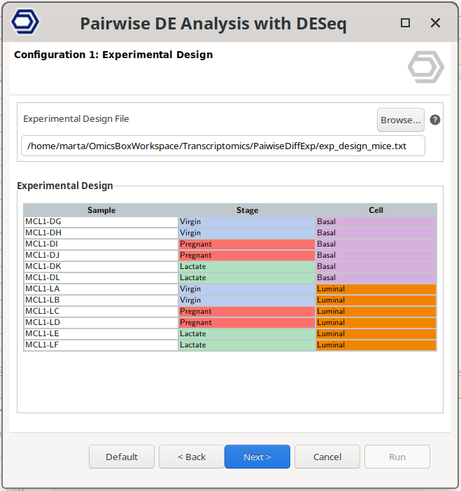
Figure 5: Experimental Design Page
Filtering Data Page
Lowly expressed genes can introduce noise and reduce the reliability of statistical modeling. This section allows removing genes with insufficient counts across samples before running the differential expression analysis.
-
Samples Reaching Filter: Defines the minimum number of samples in which a gene must pass the selected count threshold. For example, if this value is set to 5, the gene must have expression above the selected filter value in at least 5 samples. A common practice is to use the number of samples in the smallest experimental group. For example, if one condition has 2 replicates and another has 3, the filter is typically set to 2, meaning that a gene must be expressed in at least two samples to be retained. Set this value to 0 to disable filtering.
-
Counts Per Million (CPM): Filtering based on counts per million (CPM) accounts for differences in sequencing depth between samples. For example, a CPM of 1 corresponds to 6 counts in a sample with 6 million reads.
- CPM Filter: Minimum CPM required for a gene to be retained. Genes with CPM values below this threshold in the specified number of samples will be removed. Set to 0 to disable this filter.
-
Total Counts. Filtering based on raw read counts.
- Counts Filter: Genes with fewer counts than this value in at least the specified number of samples will be removed.
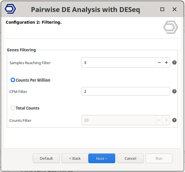
Figure 6: Filtering Data Page
Differential Expression Test Page
This page defines the statistical model used to test for differential expression. The model determines which samples are compared and how experimental factors are incorporated into the analysis. Depending on the complexity of the experiment, three design types are available.
Diffexp Design Type
-
Simple Design: The Simple Design performs a standard comparison between conditions within a single experimental factor. Genes are tested for differential expression between the selected Primary Test Condition(s) and Primary Reference Condition(s). Only the Primary Target parameters are used in this design.
Example use case:
Comparing Tumor samples (Primary Test Condition) vs Normal samples (Primary Reference Condition). If the samples were processed in different batches, a Blocking Factor such as "Batch" can be included to remove batch-associated variation before performing the Tumor vs Normal comparison. -
Multifactorial Design: The Multifactorial Design evaluates the combined effect of two experimental factors: a Primary Factor and a Secondary Factor. In this design, samples that belong to both the Primary Test Condition(s) and the Secondary Test Condition(s) are compared against samples that belong to both the Primary Reference Condition(s) and the Secondary Reference Condition(s). The test therefore compares groups defined by the combination of both factors.
Example use case:
Given an experiment with two factors: "Genotype", with "WT" and "Mutant" contidions, and "Treatment", with "Control" and "Treated" conditions, this design can compare Mutant + Treated samples against WT + Control samples.A Blocking Factor may also be included to account for additional sources of variation.
-
Interaction Design: The Interaction Design evaluates whether the effect of the Primary Factor depends on the Secondary Factor. Instead of directly comparing groups, this test evaluates an interaction term, which represents a difference of differences. It identifies genes whose response to the primary condition changes depending on the secondary background.
Example use case:
Testing whether the effect of a "Treatment" (Treated vs Control) depends on the Genotype (Mutant vs WT).This test compares the treatment effect in Mutant samples against the treatment effect in WT samples. Genes identified by this test show different responses to the treatment depending on genotype.
A Blocking Factor can also be included.
Comparison of Diffexp Design Types
| Design Type | What is Tested | Factors Used | Typical Question |
|---|---|---|---|
| Simple Design | Direct comparison between two conditions | Primary Factor only | Which genes differ between Condition A and Condition B? |
| Multifactorial Design | Comparison of groups defined by two factors together | Primary + Secondary Factors | Which genes differ between a specific combination of conditions (e.g., Mutant + Treated vs WT + Control)? |
| Interaction Design | Whether the effect of one factor depends on another | Primary + Secondary Factors | Does the effect of Treatment differ between Genotypes? |
Blocking Factor
- Blocking Factor: Select a factor that may introduce technical or unwanted biological variation, such as batch, sequencing lane, or patient ID. The variation associated with this factor is incorporated into the statistical model so that it does not confound the main comparison. This allows the differential expression test to focus on the factors of interest. If no such factor exists, select None.
Primary Target
The Primary Target defines the main comparison of interest.
- Primary Factor: Select the experimental factor that defines the primary comparison.
- Primary Test Conditions: Select the condition(s) that will form the test group. If multiple conditions are selected, they are combined and their effect is averaged during the statistical comparison.
- Primary Reference Conditions: Select the condition(s) that will form the reference group. If multiple conditions are selected, their effect is also averaged.
Secondary Target
The Secondary Target defines an additional experimental factor used in Multifactorial and Interaction designs.
- Secondary Factor: Select the secondary experimental factor.
- Secondary Test Conditions: Select the condition(s) defining the test state for the secondary factor. If multiple conditions are selected, they are combined and their effect is averaged during the statistical comparison.
- Secondary Reference Conditions: Select the condition(s) defining the reference state for the secondary factor. If multiple conditions are selected, their effect is also averaged.
Depending on the selected design:
- In a Multifactorial Design, the secondary factor helps define the combined groups that are compared.
- In an Interaction Design, the secondary factor determines the background in which the primary effect is evaluated.
Understanding Primary and Secondary Targets
The Primary Target always defines the main biological effect you want to measure, while the Secondary Target provides additional experimental context.
Simple Design Example
- Primary Factor: Condition
- Primary Test Conditions: Tumor
- Primary Reference Conditions: Normal
→ Comparison performed: Tumor vs Normal
Multifactorial Design Example
- Primary Factor: Genotype
- Primary Test Conditions: Mutant
- Primary Reference Conditions: WT
- Secondary Factor: Treatment
- Secondary Test Conditions: Treated
- Secondary Reference Conditions: Control
→ Comparison performed: (Mutant + Treated) vs (WT + Control)
Interaction Design Example
- Primary Factor: Treatment
- Primary Test Conditions: Treated
- Primary Reference Conditions: Untreated
- Secondary Factor: Genotype
- Secondary Test Conditions: Mutant
- Secondary Reference Conditions: WT
→ Comparison performed: (Treated + Mutant vs. Untreated + Mutant) - (Treated + WT vs. Untreated + WT)
→ This tests whether: Treatment effect in Mutant ≠ Treatment effect in WT
Statistical Test
DESeq2 always reports a log2 fold change for the comparison configured in the wizard. However, the p-value column is only guaranteed to refer to that same comparison when using the Wald test. With LRT, the p-value answers a model-comparison question that may involve all levels of a factor, not only the two levels named in the contrast.
-
Wald significance test. Tests the null hypothesis that the chosen contrast is zero (e.g. expression in the test condition equals expression in the reference condition, after accounting for the fitted design). The reported P-Value and FDR refer to that contrast.
When to use it (recommended default for this tool): Use Wald whenever the biological question is “is this specific comparison different from zero?”. -
Likelihood ratio test (LRT). DESeq2 fits a full model and a reduced model and performs a likelihood ratio test on the difference between those models (see the DESeq2 vignette, sections on the likelihood ratio test and on contrasts). Important for simple and multifactorial designs: If a factor has more than two levels, the default LRT (reduced vs full model including that factor) tests whether expression depends on that factor in general (an omnibus test over all levels). The table can still show a logFC for the chosen pairwise (or joint) contrast, but the P-Value / FDR are from the omnibus LRT, not from a pairwise test of that logFC alone. For a pairwise question with many levels, prefer Wald unless you intentionally want this global test.
When LRT is appropriate:- Simple design: Use LRT when the question is whether the primary factor as a whole explains expression (any level differs from the others under the fitted model), or when the experimental factor truly has only two levels (then the omnibus LRT aligns with that single comparison).
- Multifactorial design: LRT can test whether adding the primary factor, the secondary factor, or both (according to the fitted full vs reduced formula) significantly improves the fit globally. Again, this is not the same as a single Wald contrast p-value unless the model reduction is chosen to match that hypothesis.
- Interaction design: LRT is used to assess interaction (whether the effect of one factor depends on the other) according to the reduced model documented in the DESeq2 workflow for this analysis type.
For precise pairwise or contrast-specific inference with several factor levels, Wald is usually the safer choice.
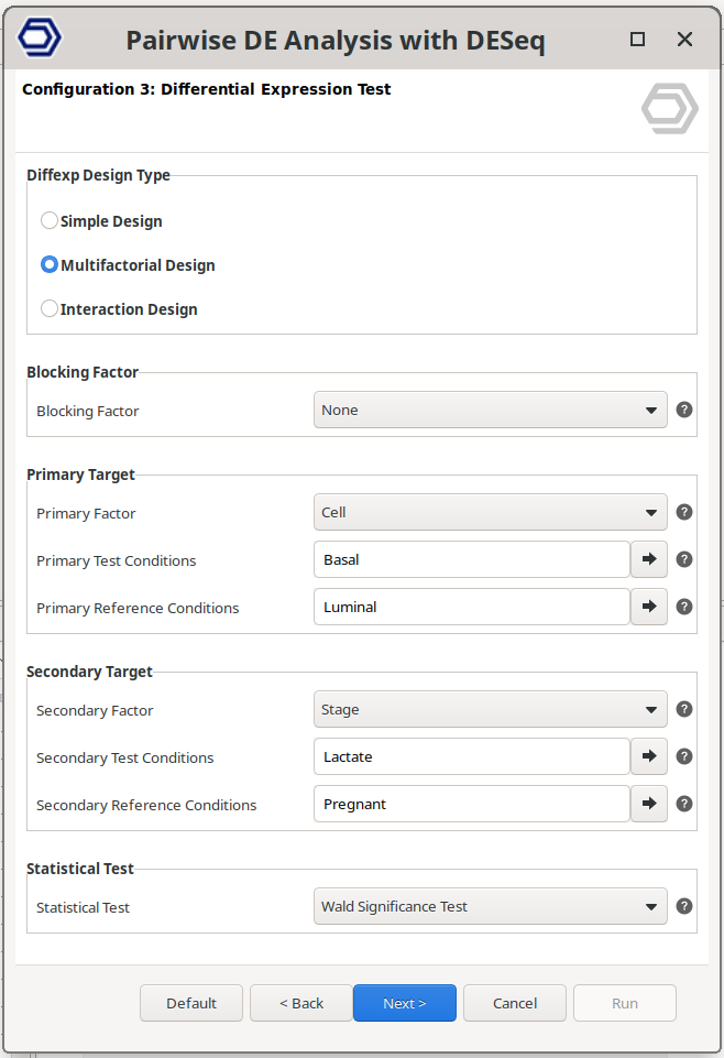
Figure 7: Differential Expression Test Page.
Results
Main Viewer
Once the analysis finishes, a new tab is opened containing the main results (Figure 8). The results table contains the differential expression statistics, where each row corresponds to a feature. Genes that have not passed the filtering step are not shown in the new tab.
- Tags: Indicate whether a gene is significantly UP (FDR ≤ 0.05 and logFC ≥ 0) or DOWN (FDR ≤ 0.05 and logFC ≤ 0) regultated. These are the default thresholds, which can be updated from the Side Panel.
- Feature: Identifier of the genomic feature (gene, transcript, or other feature). This corresponds to the IDs provided in the input count table.
- Base Mean: Mean of the normalized counts for the feature across all samples. Normalization accounts for differences in library size between samples.
- lfcSE: Standard error of the log2 fold change estimate. This value reflects the uncertainty of the estimated fold change.
- logFC: Log2 fold change between the test and reference conditions defined in the experimental design. Positive values indicate higher expression in the test condition, while negative values indicate higher expression in the reference condition.
- FDR: False Discovery Rate (adjusted p-value) obtained using the Benjamini–Hochberg correction. This value controls for multiple testing across all analyzed genes.
- P-Value: Raw p-value obtained from the statistical test before multiple-testing correction.
- Stat: Value of the test statistic used to compute the p-value. Its interpretation depends on the selected statistical test:
- Wald Test: The statistic corresponds to the Wald statistic, calculated as the estimated log2 fold change divided by its standard error. Larger absolute values indicate stronger evidence for differential expression.
- Likelihood Ratio Test (LRT): The statistic corresponds to the difference in deviance between the full and reduced models, which follows a chi-squared distribution. Larger values indicate that the removed factor significantly contributes to explaining the gene's expression variation.
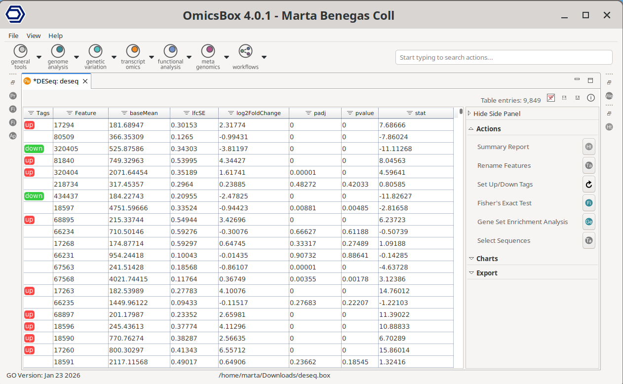
Figure 8: Pairwise Differential Expression Results
Side Panel
Actions
Summary Report
It generates the Summary Report of the analysis (Figure 9).
The Dataset Overview section contains a summary of the gene filtering and the total number of samples included in the analysis.
The Results section contains the total number of differentially expressed features, and how many are up and how many are down regulated. It also shows the current thresholds to call a feature differentially expressed.
The Experimental Design section shows the current experimental design, as well as the total library size per sample, that is, it's total number of counts pre and post filtering.
Finaly, the Analysis Parameters and the References are listed.
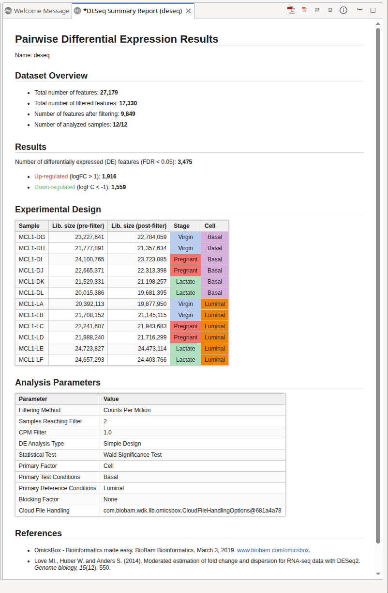
Figure 9: Results Summary
Rename Features
This option allows modifying the sequence IDs in the Feature column using different methods:
- Add: Add a prefix or sufix to all IDs in the table.
- Replace: Replace specific text within the IDs. The text to be replaced must be defined in the Find parameter using a regular expression (regex).
- Mapping: Use a mapping file to rename features. The mapping file must be a tab-separated text file with two columns: the first column contains the original feature IDs from the dataset, and the second column contains the new feature names. If duplicate IDs occur during renaming, you can define how they are handled:
- Sum Rows: Combine counts for all matching features.
- First Row: Retain only the counts of the first occurrence.
Set Up/Down Tags
It re-assigns the UP and DOWN labels based on different filtering cutoffs (Figure 10). Tags will be updated, and the result section of the Result Summary and statistical charts will change according to the new cutoffs.
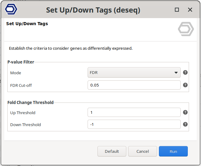
Figure 10: Set Up/Down Tags
Fisher's Exact Test
Fisher’s Exact Test can be used to find GO terms that are over and under-represented in a set of genes (test set) with respect to a reference group (reference set). Fisher’s Exact Test uses a contingency table-based method to examine the association between two kinds of classification. There’s more information about the analysis and the parameters in the Fisher's Exact Test section.
With this tool, the subset of genes that will be considered as a Test-set will be the genes labeled as UP or DOWN regulated (Figure 11). Up-regulated and down-regulated genes are those that are tagged according to the criteria established by the option "Set Up/Down Tags".
The project containing the functionally annotated sequences that will be used as a reference background set should be provided in the "Reference Annotation" box.
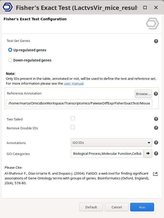
Figure 11: Fisher’s Exact Test
Gene Set Enrichment Analysis
Gene Set Enrichment Analysis (GSEA) is a computational method that determines whether an a priori defined set of genes shows statistically significant, concordant differences between two biological states (e.g. phenotypes). There’s more information about the analysis and the parameters in the Gene Set Enrichment Analysis section.
This analysis needs a ranked gene list, which will be automatically computed using the following formula:
Rank = sign(logFC) * -log10(P-Value)
The project containing the functionally annotated sequences that will be used as a reference background set should be provided (Figure 12).
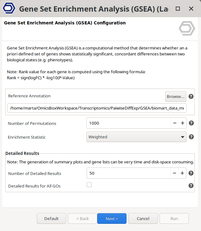
Figure 12: Gene Set Enrichment Analysis
Charts
Different statistics charts can be generated for a global visualization of the results. These charts can be found under the Side Panel → Chartsof the Pairwise Results viewer.
Results Chart
Bar chart which shows the total number of features, kept features (those who have passed the filtering step), differentially expressed features, up-regulated features, and down-regulated features (Figure 13).
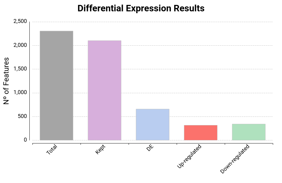
Figure 13: Result Summary
MDS Plot
Generates a two-dimensional scatterplot in which the distances represent the typical log2 fold changes between samples. You can select an experimental factor by which you want to color the MDS graphic (Figure 14).
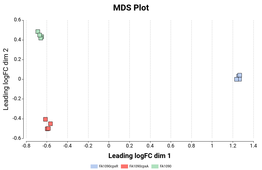
Figure 14: MDS Plot
Volcano Plot
A scatter plot constructed by plotting the negative log of the adjusted p-values (FDR) on the y-axis versus the log of the fold changes on the x-axis (Figure 15). Upregulated and downregulated genes are shown in green and red respectively.
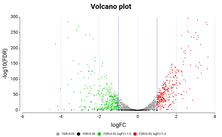
Figure 15: Volcano Plot
Heatmap
A heatmap is a two-dimensional visualization in which numerical values are represented using a color scale (Figure 16). In the context of differential expression analysis, heatmaps are commonly used to visualize the expression patterns of selected genes across all samples.
The rows represent genes, while the columns represent samples. The color of each cell reflects the expression level of a gene in a given sample, allowing patterns such as co-expression or sample similarity to be easily identified.
The dendrograms displayed on the left (genes) and top (samples) are generated using hierarchical clustering based on the Euclidean distance between expression profiles. This clustering groups together genes with similar expression patterns and samples with similar transcriptomic profiles.
The heatmap supports interactive zooming. Users can zoom into a specific cluster by clicking and holding a node in either dendrogram.
The bars shown above the heatmap represent the experimental design factors, illustrating how each sample is associated with the experimental covariates (e.g., condition, treatment, batch).
The features to be displayed can be selected in the wizard via the Select Features parameter:
- Top 50 differentially expressed genes, ranked by FDR.
- All differentially expressed genes.
- Custom gene list, provided as a list of feature IDs.
Note: Differentially expressed genes are those labeled as UP or DOWN in the project table (column Tags). The thresholds used to classify genes as up- or downregulated can be adjusted using the option Set Up/Down Tags.
The wizard also allows users to define the expression values used for visualization with the Expression Data parameter. The heatmap can be generated using CPM values or raw counts, and additional transformations can be applied.
These transformations are useful because raw count data typically spans several orders of magnitude and is strongly influenced by highly expressed genes, which can obscure meaningful patterns in the heatmap.Available transformations include:
-
Logarithm: Reduces the dynamic range of the data, making differences among moderately expressed genes more visible and reducing the dominance of highly expressed genes.
-
Z-score: Standardizes the expression values for each gene across samples by centering the mean to zero and scaling by the standard deviation. This highlights relative expression changes between samples rather than absolute expression levels, making it easier to identify clusters of genes with similar expression patterns.
These transformations are applied only for visualization purposes and do not affect the statistical results of the differential expression analysis.
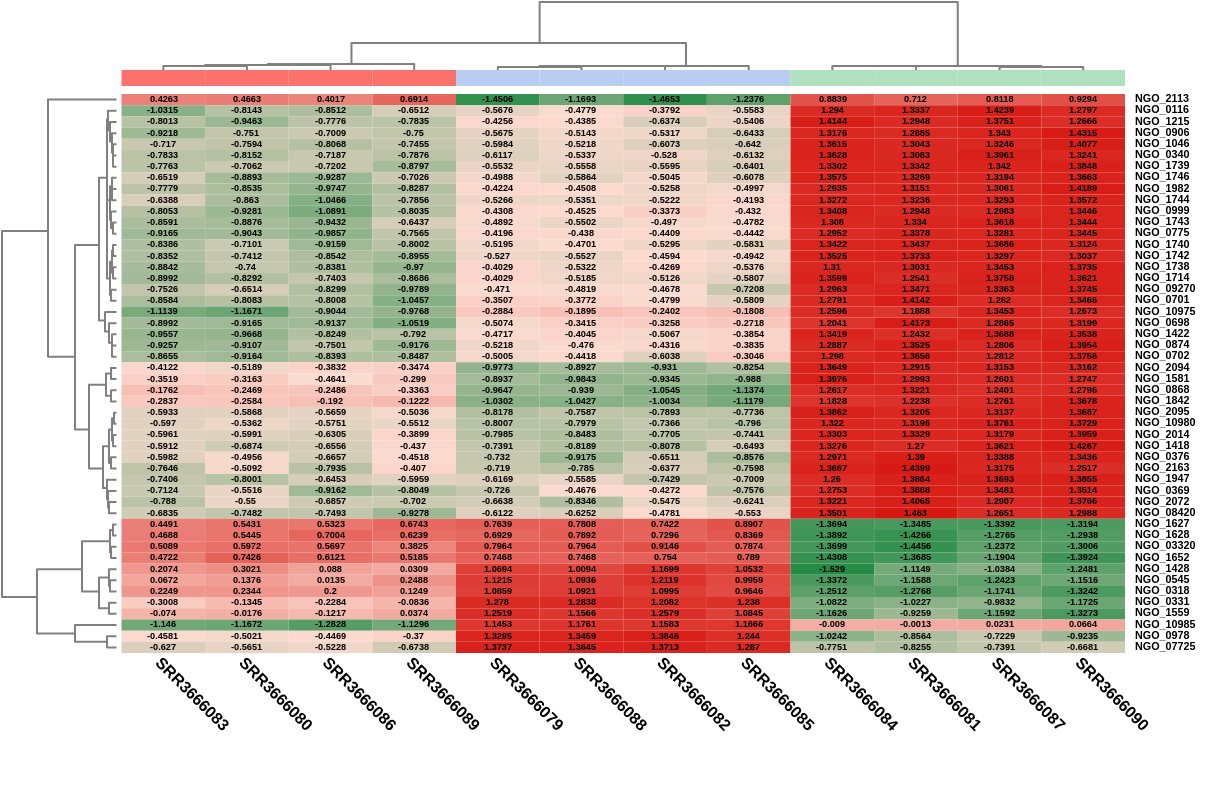
Figure 16: Heatmap
Export
Besides the generic Export Table, this object contains the following export options.
Export Raw Counts
Export the raw counts to a text file. It will not contain the genes discarded during the filtering step.
Export Experimental Desing
Esport the experimental design to a tab-separated file. The first column will contain the samples, whereas the rest will be the experimental factors.
Export Ranked List
Export a Ranked List with genes in one column and the rank in another column. Rank value for each gene is computed using the following formula: Rank = sign(logFC) * -log10(P-Value)
Context Menu
Besides the generic context menu options, the available action for this object is:
- Extract Selection to New Tab: Extract the data from the selected rows and open it in a new tab.
OmicsBox Engine
This tool can be run from the command line via the OmicsBox Engine.
Command: omicsbox deseq [options]
Input constraint: provide exactly one of:
--i-count-table,--i-count-table-file.
Inputs
| Flag | Type | Required | Description |
|---|---|---|---|
--i-design-file |
file | Yes | Experimental Design File |
--i-count-table |
file | Yes | Count Table (.box, or plain file) |
--i-count-table-file |
file | Yes | Count Table as a plain text file (.txt/.tsv/.csv) |
Parameters
| Flag | Type | Default | Range / Candidates | Required | Description |
|---|---|---|---|---|---|
--filtering-method |
enum | cpm | cpmcountsSum |
No | Filtering Method |
--minimum-samples |
integer | 2 | ≥ 0 | No | Samples Reaching Filter |
--cpm-filter |
double | 1.0 | 0.0 – 10.0 | No | CPM Filter |
--min-counts |
integer | 20 | ≥ 0 | No | Counts Filter |
--de-analysis |
enum | simple | simplemultifactorialinteraction |
No | DE Analysis Type |
--de-test |
enum | Wald | WaldLRT |
No | Statistical Test |
--primary-factor |
string | No | Primary Factor | ||
--primary-tests |
string (multiple) | No | Primary Test Conditions | ||
--primary-references |
string (multiple) | No | Primary Reference Conditions | ||
--blocking-factor |
enum | none | none |
No | Blocking Factor |
--secondary-factor |
string | No | Secondary Factor | ||
--secondary-tests |
string (multiple) | No | Secondary Test Conditions | ||
--secondary-references |
string (multiple) | No | Secondary Reference Conditions | ||
--delimiter |
enum | tab | tabspacecommasemicolon |
No | |
--na-treatment |
enum | skip | skipzero |
No |
Parameter relationships
| Flag | When | Effect | Affected flags |
|---|---|---|---|
--filtering-method |
countsSum |
disables | --cpm-filter |
--filtering-method |
countsSum |
enables | --min-counts |
--de-analysis |
multifactorial |
enables | --secondary-factor |
--de-analysis |
interaction |
enables | --secondary-factor |
Note:
--secondary-tests,--secondary-referencesare context-dependent — they apply, and their valid values are determined, only for certain input configurations.Global options (
--local-folder,--cloud-folder,--output-format,--config,--detach,--verbose, …) are shared by every Engine tool and are not repeated here — see the OmicsBox Engine reference.