Differential Abundance Analysis of Taxa
Introduction
The Differential Abundance Analysis of Taxa is a tool to identify Operational Taxonomic Units (OTUs) that significantly differ between two microbial communities. This feature is based on edgeR, which belongs to the Bioconductor project, and implements statistical tests to evaluate the significance of OTU abundances between a contrast and a reference group.
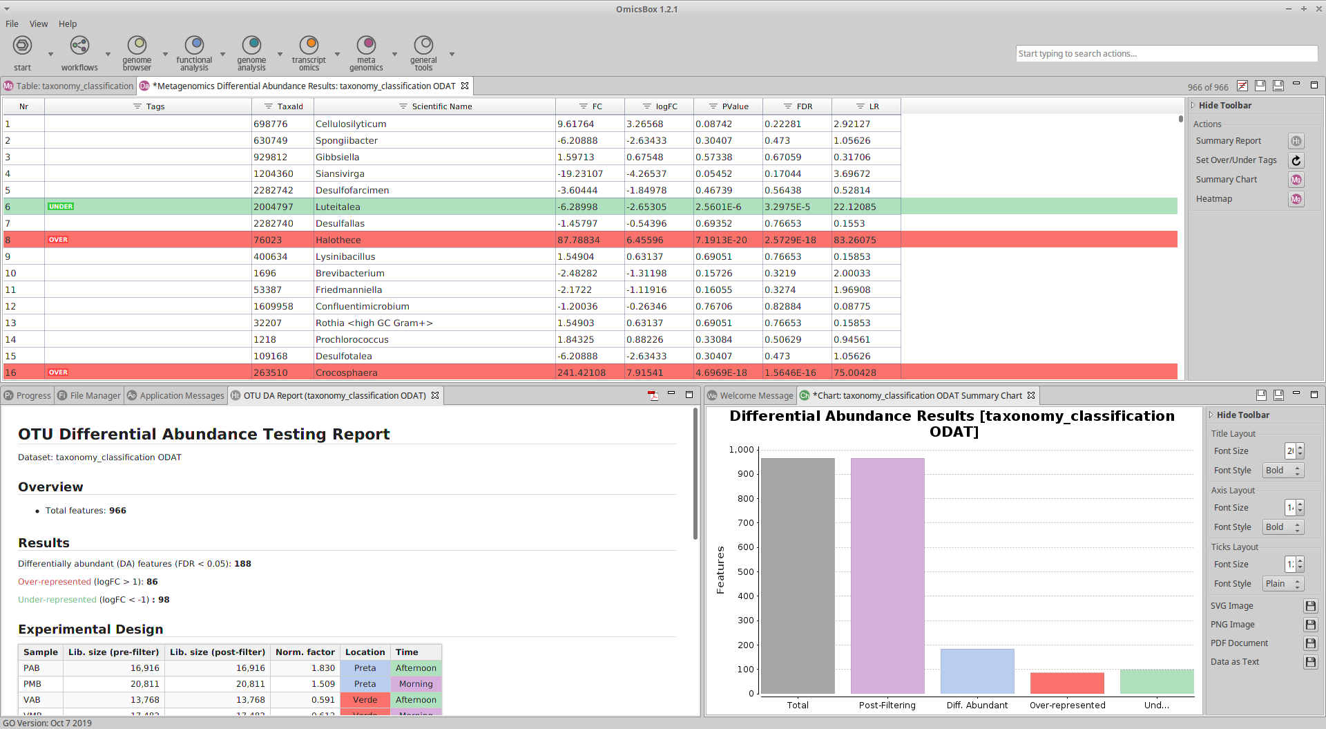
Figure 1. Differential Abundance Testing: presentation of results.
Run Differential Abundance Analysis of Taxa
With a Taxonomic Classification result opened, go to Metagenomics → Comparative Analysis → Differential Abundance Analysis of Taxa. In the wizard, you can select the parameters to run the test. It is divided into three sections: Filtering and Normalization Page (Figure 2), Experimental Design Page (Figure 3), and Statistical Test Page (Figure 5).
Filtering and Normalization Page
OTUs with low counts will not be considered for the test as they provide little evidence of differential abundance. There are two different filtering steps:
- Counts per Million Filter. Set a filter to exclude OTUs with low counts across all samples. Filtering is performed on a count-per-million (CPM) basis to account for differences in library sizes between samples (a CPM of 1 corresponds to a count of 6 in a sample with 6 million total counts). Set this value to 0 if no filtering is desired.
- Minimum Samples Filter. Set a minimum number of samples in which the CPM has to be above the previous filter. If this value is set to 5, at least 5 of the samples have to show a count above the given CPM. The number of samples of the smallest group is usually used, for example in an experiment that has 2 replicates for each condition or group, an OTU should be counted in at least 2 samples. Set this value to 0 if no filtering is desired.
In this test, the normalization takes the form of scaling factors for library sizes that enter into the statistical model. These correctional factors are used to compute the effective library sizes. 5 different options are available for the normalization step:
- TMM (Trimmed Mean of M-values). The M-values are weighted according to inverse variances and computed by the delta method for logarithms of binomial random models.
- TMMwsp (TMM with singleton pairing). This is a variant of TMM that is intended to perform better for data with a high proportion of zeros (default).
- RLE (Relative Log Expression). Scale factors are the median ratio of each sample to the median library, the geometric mean of all samples.
- Upper-quartile. 75% quantiles for the counts of each library are used to calculate the scale factors.
- None. All normalization factors are set to 1.
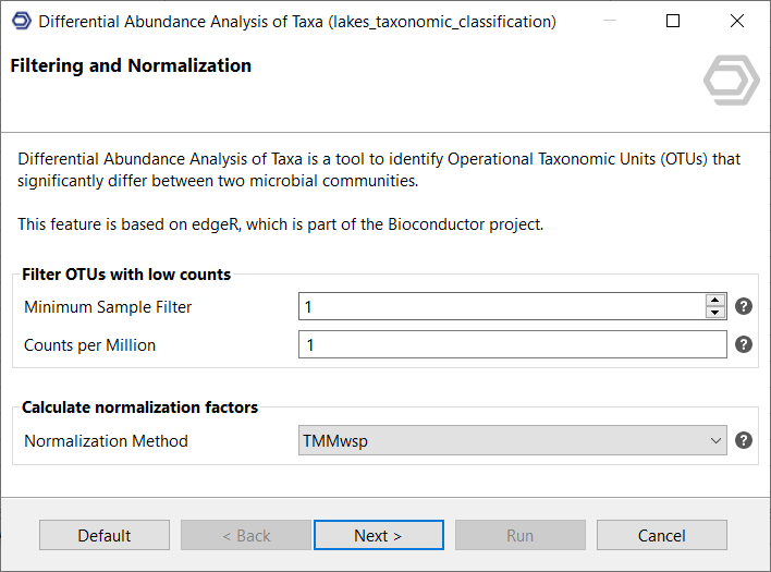
Figure 2. Differential Abundance Testing wizard: filtering and normalization page.
Experimental Design Page
Here, the two groups for the test, reference and contrast, have to be specified. You can select the groups by choosing which samples from the taxonomic classification project you want to include in each one, or by loading an experimental design file and selecting the conditions you want to test.
Select samples (no experimental design file loaded)
Select the samples to be considered for the test and divide them into two groups or conditions. The Contrast Group will be the samples that will be tested against the Reference Group.
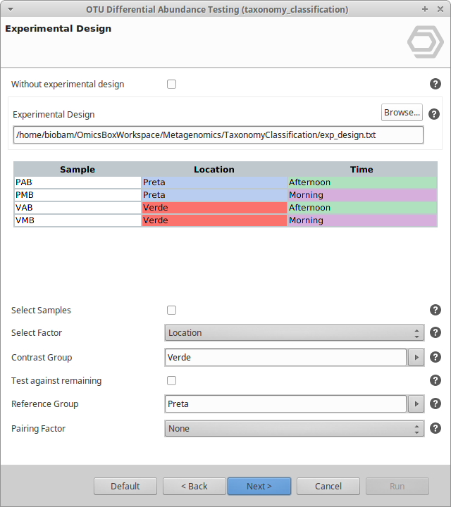
Figure 3. Differential Abundance Testing wizard: experimental design page.
Experimental design file
You can load your experimental design file. This file must contain the sample names in the first column and the experimental conditions of each sample in the following ones, as can be seen in Figure 4. Please make sure the sample names in the first column of this experimental design file match exactly with the samples in the taxonomic classification result.
This experimental design file must be in tsv format (tab-separated values file). In this kind of file, each field is separated with a tab character. Please do not use spaces and avoid unusual characters when writing your experimental design file, to be sure that it will be correctly read and processed.
Once the file is properly loaded, you can select an experimental factor from the experimental design and the conditions to test in both the Contrast and Reference groups. You can also select samples separately as described in the previous section if the Select Samples option is checked.
If a paired design is desired, a Pairing Factor from the experimental design can be optionally selected to adjust for the baseline difference of this factor. Note that this option is only available if you have provided an experimental design file.
Experimental design example
Sample  Lake    Time
PAB Preta   Afternoon
PMB Preta   Morning
VAB Verde   Afternoon
VMB Verde   Morning
Figure 4. Experimental design file.
Statistical Test Page
You can Test at Specific Taxonomic Levels to only consider results for a specific taxon, such as species, genus, or family.
Here, you can select the statistical test to be used to detect the differentially abundant OTUs. The test assumes that the OTU counts across groups are distributed as negative binomial random variables. Two different kinds of tests are available:
- Exact Test. Run an Exact Test to detect a difference in mean between two groups of OTU abundance libraries, reference and contrast groups. This test is performed for each OTU and can only be used if no pairing factor is selected.
- Generalized Linear Model. Fit a negative binomial generalized log-linear model (GLM) to the counts for each OTU. Two different GLM tests are allowed:
- GLM Likelihood Ratio Test. This mode conducts likelihood ratio tests for the coefficients in the linear model using the Cox-Reid dispersion estimates.
- GLM Quasi Likelihood F-Test. It is similar to the LRT test, except that it replaces likelihood ratio tests with empirical Bayes quasi-likelihood F tests. This test provides a more robust and reliable error rate control when the number of replicates is small.
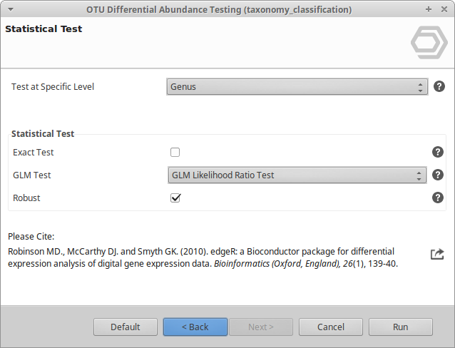
Figure 5. Differential Abundance Testing wizard: statistical test page.
Results
Once the taxonomic abundance analysis has finished, a new table with the results will open (Figure 6). Each row of this table corresponds to a different tested OTU. Each column contains:
- Tags. Indicate if a specific OTU is overrepresented, tag OVER, with FDR below 0.05 and logFC above 1, or underrepresented, tag UNDER, with FDR below 0.05 and logFC below -1, in the contrast sample.
- FC (Fold Change). The ratio between the mean abundance value of a specific OTU in the contrast condition and this value in the reference condition, if the mean abundance value in the contrast group is bigger than in the reference group. If this value is bigger in the reference group, then the FC is calculated as the ratio between the mean abundance value in the reference condition and the value in the contrast condition with a negative sign. By default, an OTU is defined as overrepresented if FC is above 2, and underrepresented if FC is below -2.
- LogFC. The log2 FC. By default, an OTU is defined as overrepresented if logFC is above 1, and underrepresented if logFC is below -1, if it is statistically significant, FDR below 0.05 by default.
- LR (Likelihood Ratio). Likelihood Ratio statistic for the GLM, only if the GLM LR test is selected.
- F. Quasi-likelihood F-statistic for the GLM, only if the GLM QL test is selected.
- P-value. The p-value for the null hypothesis of non-differential abundance.
- FDR. A corrected p-value for multiple testing comparisons (Benjamini Y., Hochberg Y., 1995). If meeting the logFC criterion, logFC above 1 or below -1 by default, an OTU must have an FDR below 0.05 to be considered as differentially abundant.
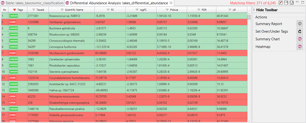
Figure 6. OTU Differential Abundance Testing results.
Side panel
Summary Report
Creates an HTML report which can be saved in PDF with the main results of the Differential Abundance Testing: parameters used for the test, number of differentially abundant OTUs, experimental design, and other details (Figure 7).
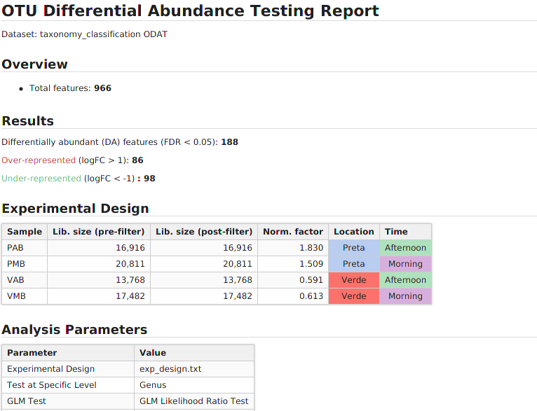
Figure 7. OTU Differential Abundance Testing summary report.
Summary Chart
Shows a bar chart with the main results: OTUs pre and post filtering steps, OTUs that are considered as differentially abundant, and the over- and underrepresented ones (Figure 8).
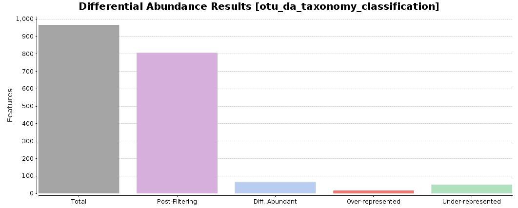
Figure 8. OTU Differential Abundance Testing summary chart.
Set Over/Under Tags
Establish a new FDR and Fold Change cutoff to consider OTUs as differentially abundant. FDR below 0.05 and logFC below -1 or above 1 are set as default (Figure 9).

Figure 9. Set Over/Under Tags.
Heatmap
Shows a two-dimensional heatmap in which the abundance values are represented by ranges of colors (Figure 10). The dendrograms added to the left and top side are produced by a hierarchical clustering method that takes as input the Euclidean distance computed between OTUs, on the left, and samples, on top.
The upper bars show the experimental conditions of the study, as columns, and the OTU names are shown at the right of each row.
You can select if you want to draw the heatmap with the raw counts or with the CPM values, and if any transformation is necessary: logarithm in base 2, Z-score, or both.
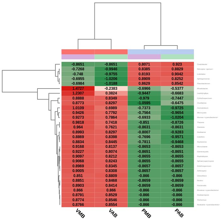
Figure 10. Heatmap.
OmicsBox Engine
This tool can be run from the command line via the OmicsBox Engine.
Command: omicsbox odat [options]
Inputs
| Flag | Type | Required | Description |
|---|---|---|---|
--i-experimental-design |
file | No | Experimental Design |
--i-tcresult |
file | Yes | Taxonomic Classification |
Parameters
| Flag | Type | Default | Range / Candidates | Required | Description |
|---|---|---|---|---|---|
--level |
enum | species | classorderfamilygenusspecies |
No | Test at Specific Level |
--mode |
enum | GLM_LRT | GLM_LRTGLM_QL |
No | GLM Test |
--robust |
boolean | true | No | Robust | |
--normalization |
enum | tmmwsp | tmmwsptmmupperquartilerlenone |
No | Normalization Method |
--samples |
integer | 1 | 0 – 500 | No | Minimum Sample Filter |
--cpm |
double | 1.0 | 0.0 – 10.0 | No | Counts per Million |
--exact-test-mode |
boolean | false | No | Exact Test | |
--pairing-factor |
enum | No_Design | No_Design |
No | Pairing Factor |
--against-the-rest |
boolean | true | No | Test against remaining | |
--select-factor |
enum | No_Design | No_Design |
No | Select Factor |
--select-samples |
boolean | true | No | Select Samples | |
--design |
boolean | false | No | Experimental design | |
--exclude-not-selected-samples |
boolean | false | No | Exclude not selected samples | |
--contrast-group |
string (multiple) | No | Contrast Group | ||
--ref-group |
string (multiple) | No | Reference Group |
Parameter relationships
| Flag | When | Effect | Affected flags |
|---|---|---|---|
--exact-test-mode |
true |
disables | --mode |
--against-the-rest |
false |
enables | --ref-group |
--design |
true |
enables | --i-experimental-design, --select-samples |
--design |
true |
disables | --exact-test-mode |
Note:
--pairing-factor,--select-factorare context-dependent — they apply, and their valid values are determined, only for certain input configurations.Global options (
--local-folder,--cloud-folder,--output-format,--config,--detach,--verbose, …) are shared by every Engine tool and are not repeated here — see the OmicsBox Engine reference.
References
Robinson MD, McCarthy DJ and Smyth GK (2010). "edgeR: a Bioconductor package for differential expression analysis of digital gene expression data." Bioinformatics, 26, pp. -1.