Differential Expression Analysis with limma
Introduction
This tool performs differential expression analysis on RNA-seq counts, quantitative proteomics intensities (label-free, TMT/iTRAQ, DIA/DDA) and microarray data. It is based on the limma Bioconductor package, extended with edgeR/voom for RNA-seq counts and DEqMS for peptide/PSM-count-aware variance modeling of mass-spectrometry proteomics data.
The software package limma, part of the Bioconductor project, fits a linear model to each feature and applies empirical Bayes moderation of the variance across all features. This borrows information across the whole dataset to stabilize variance estimates, which is particularly valuable with small sample sizes. RNA-seq raw counts are first transformed with voom, which converts counts to log2-counts-per-million and estimates precision weights that account for the count mean-variance relationship, after which they are analyzed with the same linear-model framework used for intensities and microarray data. For mass-spectrometry proteomics, an optional DEqMS step further adjusts the variance estimate of each protein according to the number of peptides/PSMs used to quantify it, addressing the fact that proteins quantified from fewer peptides have less reliable variance estimates.
When the DEqMS statistical model is used, please also cite: Zhu Y, Orre LM, Zhou Tran Y, et al. (2020). DEqMS: A Method for Accurate Variance Estimation in Differential Protein Expression Analysis. Molecular & Cellular Proteomics, 19(6), 1047-1057. https://doi.org/10.1074/mcp.TIR119.001646
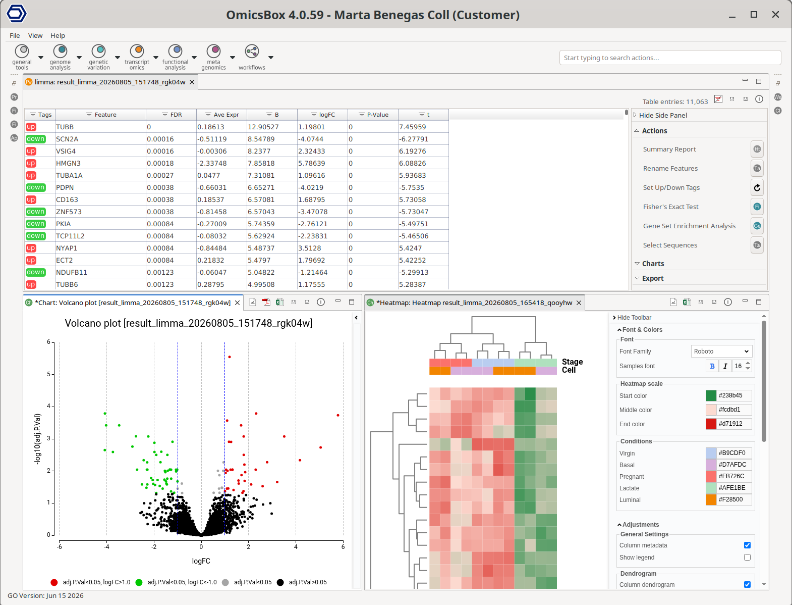
Figure 1: Differential Expression Analysis Interface
Expression Data
The analysis expects feature-level quantification data in the form of a count table: raw read counts for RNA-seq, or protein/peptide intensities, ratios or spectral counts for proteomics and microarray data.
RNA-seq count tables can be generated with the Create Count Table application. Protein/peptide quantification tables, as well as RNA-seq count tables, can also be imported from a text file. Go to transcriptomics → Load → Load RNA-Seq / Protein Quantification Count Table (Figure 2) and select the file containing the table.
On this wizard, the Data Type parameter must be set to match the type of data being loaded:
- RNA-Seq: Raw read counts. The default treatment for missing values is Skip Line, since a missing value in raw counts is usually the result of an upstream error.
- Protein: Quantification values, such as intensities or peptide/PSM counts. The default treatment for missing values is Assume Zeros, since missing values are common in proteomics data and typically represent a feature that was not detected, rather than an upstream error. When this option is selected, the resulting zeros should later be treated as missing again in the limma wizard (see Data Type & Preprocessing below), so that they are handled correctly rather than analyzed as a genuine zero measurement.
Notes:
- This application only accepts raw counts or quantification values, without any prior normalization.
- Replicates for each experimental condition are mandatory. For RNA-seq experiments without replicates, use the Pairwise Differential Expression Analysis (Without Replicates) option instead.
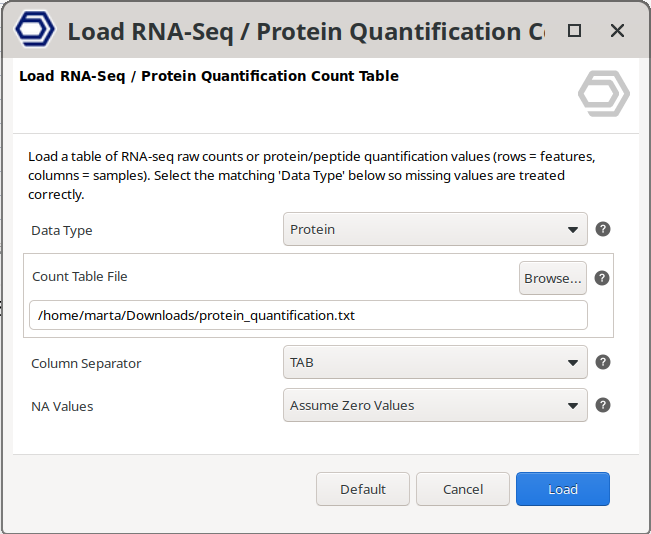
Figure 2: Load Count Table from File
Run Differential Expression Analysis with limma
Go to transcriptomics → Differential Expression Analysis. The first wizard page (Figure 3) is always the selection of the differential expression method; choose the "Limma" option.
If no count table is currently loaded in OmicsBox, the next wizard page (Figure 4) asks to provide either a Count Table Project (.box file) or a Count Table File (.txt, .csv, or .tsv file), together with the treatment of missing values. When "Limma" is selected on the previous page, this value defaults to "Assume Zeros", since limma is the only method among those offered here that can analyze proteomics/microarray intensities, where missing values are common. If a count table is already loaded in OmicsBox (see Expression Data above), this page is skipped and the one already loaded is used directly. The analysis can also be started from Side Panel → Actions → Differential Expression Analysis on an existing count table.
After this, the limma-specific wizard pages follow, where the analysis parameters are specified.

Figure 3: Differential Expression method selection wizard page.
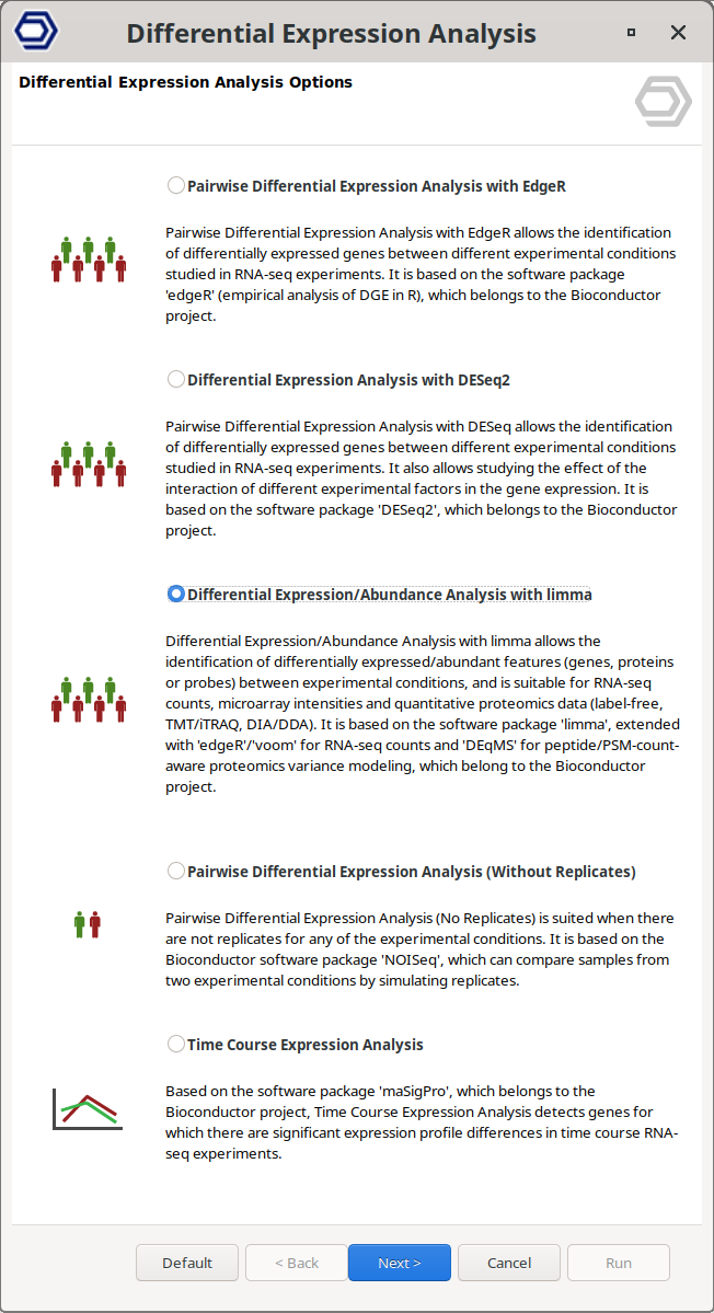
Figure 4: Input wizard page.
Experimental Design Page
- Experimental Design File: Select a .txt file containing experimental factors with the experimental conditions associated with each sample in tab-delimited format. As shown below, rows correspond to samples and columns to experimental factors. Make sure that the names in the first column of the experimental design table are exactly the same as the sample names in the count table header. If the experimental design file has fewer samples than the count table, only the samples contained in this file are analyzed.
Name    Condition
Sample1 Control
Sample2 Control
Sample3 Control
Sample4 Treated
Sample5 Treated
Sample6 Treated
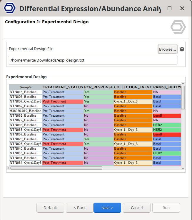
Figure 5: Experimental Design Page
Data Type & Preprocessing Page
- Input Data Type: Selects whether the loaded table contains Intensities (proteomics or microarray data) or Counts (RNA-seq raw read counts). This choice determines which of the following options apply and how the data is preprocessed.
For Intensities:
- Data Is Already Log2-Scale: Whether the input intensity values are already on a log2 scale. Disable this option when providing raw (linear-scale) intensities, so that they are log2-transformed before analysis.
- Treat Zeros As Missing: Treats zero values as missing (NA) before log2-transforming the data. This should typically stay enabled when zeros in the input table represent "not detected" features, for instance after loading a protein quantification table with the "Assume Zeros" NA treatment (see Expression Data above). It can be disabled for data types where zero is a genuine measurement, such as TMT log-ratios expressed relative to a reference channel.
- Missing Data Imputation: How to handle missing values remaining after the previous step.
- None (Let limma Handle Missing Values Natively): Recommended in most cases; limma's statistical model handles missing values without requiring imputation.
- Minimum Value Imputation (minDet): Fills missing values with a small value near each sample's detection limit. This can help when features are missing not-at-random at low intensity, i.e. when the probability of a missing value increases as the true intensity decreases.
- minDet Quantile: Quantile of each sample's observed values used to fill missing values, when Minimum Value Imputation is selected.
For Counts, the preprocessing options above do not apply; RNA-seq counts are instead transformed internally by voom (see Introduction).
- Normalization Method: Between-sample normalization method, to correct for technical differences in overall signal between samples.
For Intensities, normalization is applied on the log2 scale via limma's normalizeBetweenArrays() function (except Median, computed directly):
- Quantile (default): Forces every sample to have an identical intensity distribution. This is the strongest correction, and the standard choice for microarrays; it is also commonly used for label-free quantification (LFQ) proteomics and supports missing values natively.
- Median: Shifts each sample so that its median matches the grand median across all samples. A classic proteomics normalization, robust to missing values and to a minority of strong outliers.
- Scale: Simple linear scaling of each sample to a common median absolute deviation. A gentler alternative to Quantile.
- Cyclic Loess: Pairwise loess-based normalization that can correct intensity-dependent (non-linear) biases. It is the most computationally expensive option and is best applied on a nearly complete matrix, with few or no missing values.
- None: No normalization is applied, for example when the data has already been normalized upstream by the search engine or quantification tool.
For Counts, normalization takes the form of library-size scaling factors, computed via edgeR's calcNormFactors() before voom:
- TMM (default): Weighted trimmed mean of M-values. Recommended for most bulk RNA-seq designs.
- TMMwsp: A variant of TMM with singleton pairing, better suited to sparse data with many zero counts.
- RLE: Relative log expression (median-of-ratios). Scale factors are the median ratio of each sample to a reference computed from the geometric mean of all samples.
- Upper Quartile: The 75th percentile of the counts for each library is used to calculate the scale factors.
- None: Skips library-size normalization beyond total counts; not recommended.
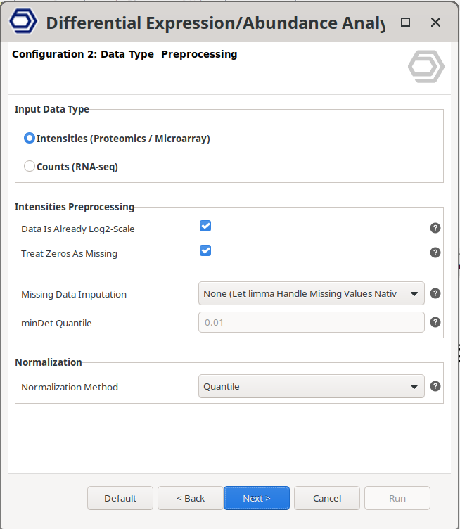
Figure 6: Data Type & Preprocessing Page
Feature Filtering Page
Lowly expressed or lowly detected features can introduce noise and reduce the reliability of statistical modeling. This section allows removing features with insufficient signal across samples before running the differential expression analysis.
- Samples Reaching Filter: Defines the minimum number of samples, within each comparison group defined by the Primary Factor, in which a feature must pass the filtering condition described below. A common practice is to use the number of samples in the smallest experimental group. Set this value to 0 to disable filtering.
For Intensities, features are filtered by their number of valid (non-missing) values per comparison group; there is no separate filtering mode to choose. For Counts, one of the following filtering modes applies:
- Counts Per Million (CPM): Accounts for differences in sequencing depth between samples.
- CPM Filter: Minimum CPM required for a feature to be retained. Features with CPM values below this threshold, in the specified number of samples, are removed.
- Total Counts: Filtering based on raw read counts.
- Counts Filter: Features with fewer counts than this value, in at least the specified number of samples, are removed.
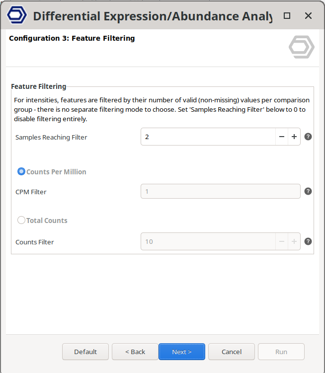
Figure 7: Feature Filtering Page
Differential Expression Test Page
This page defines the comparison to be tested and how experimental factors are incorporated into the statistical model. Depending on the complexity of the experiment, three design types are available.
Diffexp Design Type
-
Simple Design: The Simple Design performs a standard comparison between conditions within a single experimental factor. Features are tested for differential expression between the selected Primary Test Condition(s) and Primary Reference Condition(s). Only the Primary Target parameters are used in this design.
Example use case:
Comparing Tumor samples (Primary Test Condition) vs Normal samples (Primary Reference Condition). If the samples were processed in different batches, a Blocking Factor such as "Batch" can be included to remove batch-associated variation before performing the Tumor vs Normal comparison. -
Multifactorial Design: The Multifactorial Design evaluates the combined effect of two experimental factors: a Primary Factor and a Secondary Factor. Samples that belong to both the Primary Test Condition(s) and the Secondary Test Condition(s) are compared against samples that belong to both the Primary Reference Condition(s) and the Secondary Reference Condition(s). The test therefore compares groups defined by the combination of both factors.
Example use case:
Given an experiment with two factors: "Genotype", with "WT" and "Mutant" conditions, and "Treatment", with "Control" and "Treated" conditions, this design can compare Mutant + Treated samples against WT + Control samples.A Blocking Factor may also be included to account for additional sources of variation.
-
Interaction Design: The Interaction Design evaluates whether the effect of the Primary Factor depends on the Secondary Factor. Instead of directly comparing groups, this test evaluates an interaction term, which represents a difference of differences. It identifies features whose response to the primary condition changes depending on the secondary background.
Example use case:
Testing whether the effect of a "Treatment" (Treated vs Control) depends on the Genotype (Mutant vs WT).This test compares the treatment effect in Mutant samples against the treatment effect in WT samples. Features identified by this test show different responses to the treatment depending on genotype.
A Blocking Factor can also be included.
Comparison of Diffexp Design Types
| Design Type | What is Tested | Factors Used | Typical Question |
|---|---|---|---|
| Simple Design | Direct comparison between two conditions | Primary Factor only | Which features differ between Condition A and Condition B? |
| Multifactorial Design | Comparison of groups defined by two factors together | Primary + Secondary Factors | Which features differ between a specific combination of conditions (e.g., Mutant + Treated vs WT + Control)? |
| Interaction Design | Whether the effect of one factor depends on another | Primary + Secondary Factors | Does the effect of Treatment differ between Genotypes? |
Blocking Factor
- Blocking Factor: Select a factor that may introduce technical or unwanted biological variation, such as batch, sequencing lane, or patient ID. The variation associated with this factor is incorporated into the statistical model so that it does not confound the main comparison. If no such factor exists, select None.
- Blocking Mode: Only available when a Blocking Factor is selected.
- Fixed (Covariate): Spends one degree of freedom per block level. Well suited to few blocks (e.g. 2-3 batches).
- Random (duplicateCorrelation): Estimates a single within-block correlation instead of one coefficient per level. Scales better to many-level blocks (e.g. one level per patient/subject).
Primary Target
The Primary Target defines the main comparison of interest.
- Primary Factor: Select the experimental factor that defines the primary comparison.
- Primary Test Conditions: Select the condition(s) that form the test group. If multiple conditions are selected, they are combined and their effect is averaged during the statistical comparison.
- Primary Reference Conditions: Select the condition(s) that form the reference group. If multiple conditions are selected, their effect is also averaged.
Secondary Target
The Secondary Target defines an additional experimental factor, used in Multifactorial and Interaction designs.
- Secondary Factor: Select the secondary experimental factor.
- Secondary Test Conditions: Select the condition(s) defining the test state for the secondary factor. If multiple conditions are selected, they are combined and their effect is averaged during the statistical comparison.
- Secondary Reference Conditions: Select the condition(s) defining the reference state for the secondary factor. If multiple conditions are selected, their effect is also averaged.
Depending on the selected design:
- In a Multifactorial Design, the secondary factor helps define the combined groups that are compared.
- In an Interaction Design, the secondary factor determines the background in which the primary effect is evaluated.
Understanding Primary and Secondary Targets
The Primary Target always defines the main biological effect to be measured, while the Secondary Target provides additional experimental context.
Simple Design Example
- Primary Factor: Condition
- Primary Test Conditions: Tumor
- Primary Reference Conditions: Normal
→ Comparison performed: Tumor vs Normal
Multifactorial Design Example
- Primary Factor: Genotype
- Primary Test Conditions: Mutant
- Primary Reference Conditions: WT
- Secondary Factor: Treatment
- Secondary Test Conditions: Treated
- Secondary Reference Conditions: Control
→ Comparison performed: (Mutant + Treated) vs (WT + Control)
Interaction Design Example
- Primary Factor: Treatment
- Primary Test Conditions: Treated
- Primary Reference Conditions: Untreated
- Secondary Factor: Genotype
- Secondary Test Conditions: Mutant
- Secondary Reference Conditions: WT
→ Comparison performed: (Treated + Mutant vs. Untreated + Mutant) - (Treated + WT vs. Untreated + WT)
→ This tests whether: Treatment effect in Mutant ≠ Treatment effect in WT
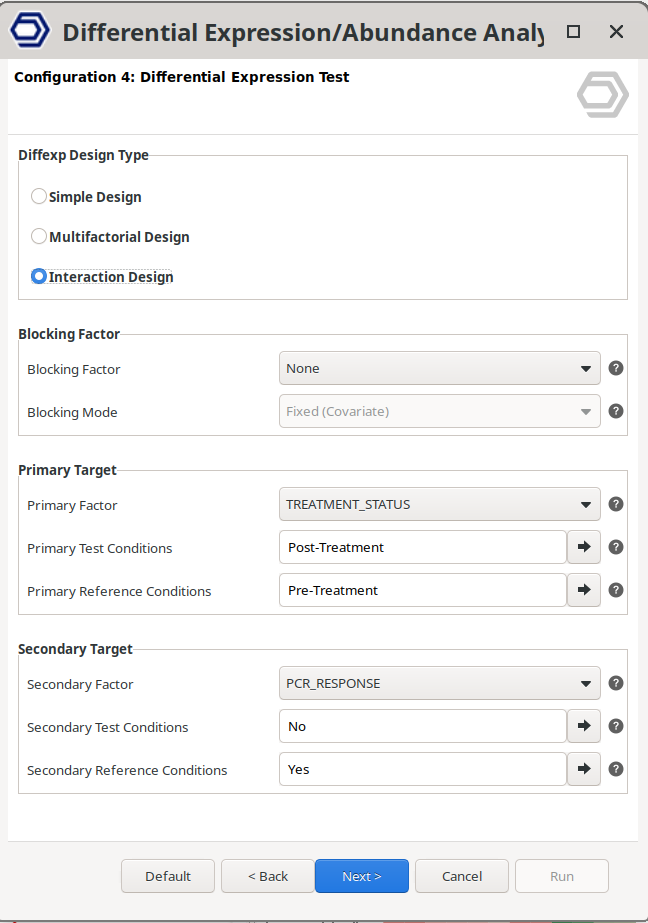
Figure 8: Differential Expression Test Page.
Statistical Model Page
- Statistical Model: Only applicable to intensities; for RNA-seq counts a note explains that the standard model is always used, since voom's precision weights already account for the count mean-variance trend.
- Standard (limma eBayes): Limma's regular empirical Bayes variance moderation.
- DEqMS (Peptide/PSM-Count-Aware): Additionally models the extra variance uncertainty of proteins quantified from few peptides/PSMs. Recommended for mass-spectrometry proteomics when a peptide/PSM count column is available.
- Peptide/PSM Count Column: Only required and available when the DEqMS statistical model is selected. Column of the input table holding the number of peptides/PSMs (or spectral counts) supporting each protein. The available options are populated automatically from the columns of the loaded count table.
- Robust Empirical Bayes: Downweights outlier features (e.g. contaminants or mis-measured proteins) when estimating the prior variance, so that a handful of extreme features cannot distort the moderation applied to every other feature. Enabled by default.
- Use Sample Quality Weights: Estimates and uses per-sample quality weights, downweighting noisy/outlier samples (
voomWithQualityWeightsfor counts,arrayWeightsfor intensities). Disabled by default. - Log2 Fold-Change Threshold: If greater than 0, tests against this minimum log2 fold-change (TREAT method) instead of testing against a null fold-change of zero. Default is 0 (disabled).
- Multiple Testing Correction: Method used to adjust p-values for multiple testing. Options are Benjamini-Hochberg (FDR, default), Benjamini-Yekutieli, Holm, Hochberg, Hommel, Bonferroni, or None.
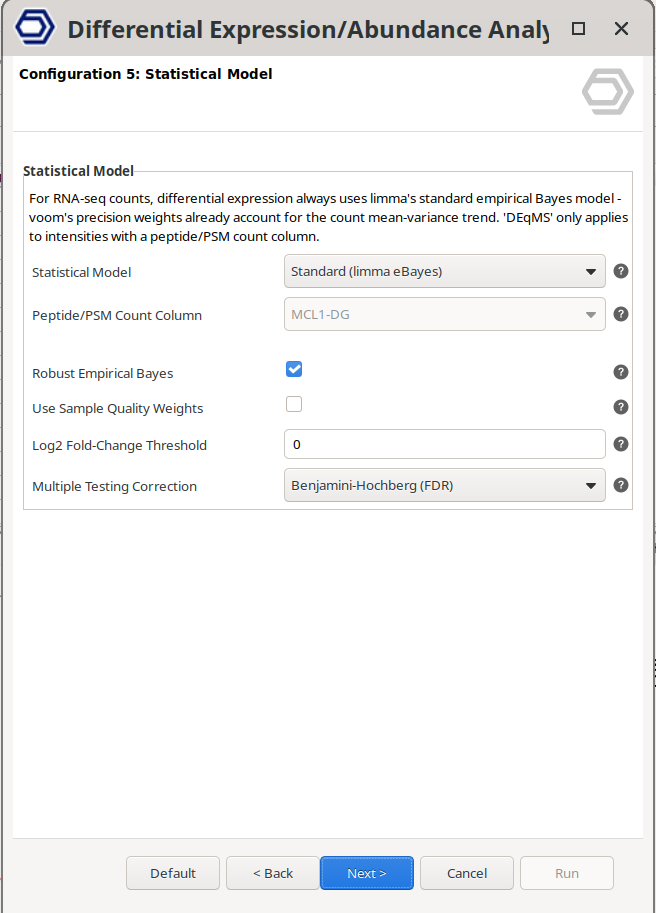
Figure 9: Statistical Model Page.
Cloud Sync Data Handling Page
This tool runs via Cloud Sync (see Cloud Sync). The last wizard page is the general CloudSync Data Handling page, where it is possible to configure where the input files are read from and where the output files are saved.
Results
Main Viewer
Once the analysis finishes, a new tab is opened containing the main results (Figure 10). The results table contains the differential expression statistics, where each row corresponds to a feature. Features that have not passed the filtering step are not shown in the new tab.
- Tags: Indicate whether a feature is significantly UP (FDR ≤ 0.05 and logFC ≥ 1) or DOWN (FDR ≤ 0.05 and logFC ≤ −1) regulated. These are the default thresholds, which can be updated from the Side Panel.
- Feature: Identifier of the feature (gene, transcript, protein, or other feature). This corresponds to the IDs provided in the input count table.
- logFC: Log2 fold change between the test and reference conditions defined in the experimental design. Positive values indicate higher expression in the test condition, while negative values indicate higher expression in the reference condition.
- Ave Expr: Average expression level of the feature across all samples, on the log2 scale used internally by limma (normalized log2 intensities for proteomics/microarray data, or log2-counts-per-million for RNA-seq). Analogous to DESeq2's "Base Mean", although on a logarithmic rather than a linear scale.
- t: Moderated t-statistic, computed as the estimated log2 fold change divided by its empirical-Bayes-moderated standard error. Larger absolute values indicate stronger evidence for differential expression. When the Log2 Fold-Change Threshold (TREAT) is greater than 0, this statistic and the associated P-Value/FDR test against that minimum fold-change rather than against zero.
- P-Value: Raw p-value obtained from the statistical test before multiple-testing correction.
- FDR: False Discovery Rate (adjusted p-value), obtained using the multiple testing correction method selected in the wizard. This value controls for multiple testing across all analyzed features.
- B: Log-odds that the feature is differentially expressed. Only available when using the standard statistical model with no Log2 Fold-Change Threshold; it is not reported by the TREAT method or by DEqMS.
When the DEqMS statistical model is used, three additional columns are shown, corresponding to the standard empirical Bayes statistics before the peptide/PSM-count-aware adjustment was applied: t (pre-DEqMS), P-Value (pre-DEqMS) and FDR (pre-DEqMS). The t, P-Value and FDR columns described above always contain the DEqMS-adjusted statistics in this case, so that these three columns remain the single, always-correct significance columns regardless of the statistical model used.
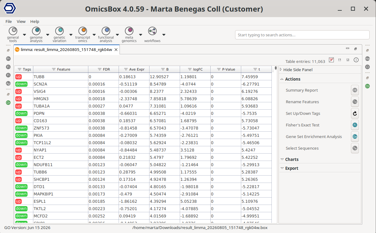
Figure 10: Differential Expression Results
Side Panel
Actions
Summary Report
Generates the Summary Report of the analysis (Figure 11).
The Dataset Overview section contains a summary of the feature filtering and the total number of samples included in the analysis.
The Results section contains the total number of differentially expressed features, and how many are up- and how many are down-regulated. It also shows the current thresholds used to call a feature differentially expressed.
The Experimental Design section shows the current experimental design, as well as the total library size (RNA-seq) or number of valid values (intensities) per sample, before and after filtering.
Finally, the Analysis Parameters and the References are listed.

Figure 11: Results Summary
Rename Features
This option allows modifying the sequence IDs in the Feature column using different methods:
- Add: Add a prefix or suffix to all IDs in the table.
- Replace: Replace specific text within the IDs. The text to be replaced must be defined in the Find parameter using a regular expression (regex).
- Mapping: Use a mapping file to rename features. The mapping file must be a tab-separated text file with two columns: the first column contains the original feature IDs from the dataset, and the second column contains the new feature names. If duplicate IDs occur during renaming, it is possible to define how they are handled:
- Sum Rows: Combine values for all matching features.
- First Row: Retain only the values of the first occurrence.
Set Up/Down Tags
Re-assigns the UP and DOWN labels based on different filtering cutoffs (Figure 12). Tags are updated, and the Results section of the Summary Report and the statistical charts change according to the new cutoffs.
- Mode: Choose between P-value or FDR (adjusted p-value) as the significance criterion.
- FDR Cut-off: P-values/FDR below this cut-off are marked with tags as up- or down-regulated. Only features that fulfill both filters (P-value/FDR and logFC) are tagged accordingly. Default value is 0.05; a value of 0 means no tags are set.
- Up Threshold: logFC values above this threshold are tagged as up-regulated. Must be greater than 0. Default value is 1, corresponding to a non-logarithmic fold change of 2.
- Down Threshold: logFC values below this threshold are tagged as down-regulated. Must be lower than 0. Default value is −1, corresponding to a non-logarithmic fold change of −2.
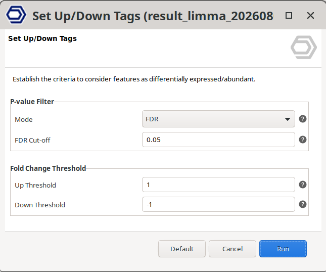
Figure 12: Set Up/Down Tags
Fisher's Exact Test
Fisher's Exact Test can be used to find GO terms that are over- and under-represented in a set of features (test set) with respect to a reference group (reference set). Fisher's Exact Test uses a contingency table-based method to examine the association between two kinds of classification. More information about the analysis and the parameters is available in the Fisher's Exact Test section.
With this tool, the subset of features considered as the Test-set are the features labeled as UP or DOWN regulated. Up- and down-regulated features are those tagged according to the criteria established by the "Set Up/Down Tags" option.
The project containing the functionally annotated sequences used as a reference background set must be provided in the "Reference Annotation" box.
Gene Set Enrichment Analysis
Gene Set Enrichment Analysis (GSEA) is a computational method that determines whether an a priori defined set of features shows statistically significant, concordant differences between two biological states (e.g. phenotypes). More information about the analysis and the parameters is available in the Gene Set Enrichment Analysis section.
This analysis needs a ranked feature list, which is automatically computed using the following formula:
Rank = sign(logFC) * -log10(P-Value)
The project containing the functionally annotated sequences used as a reference background set must be provided.
Charts
Different statistics charts can be generated for a global visualization of the results. These charts can be found under Side Panel → Charts of the Results viewer.
Result Chart
Bar chart which shows the total number of features, kept features (those that have passed the filtering step), differentially expressed features, up-regulated features, and down-regulated features.
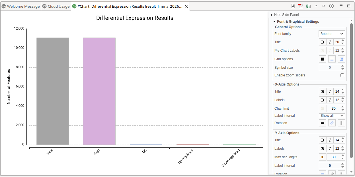
Figure 13: Result Chart
MDS Plot
Generates a two-dimensional scatterplot in which the distances represent the typical log2 fold changes between samples. An experimental factor can be selected to color the MDS graphic.
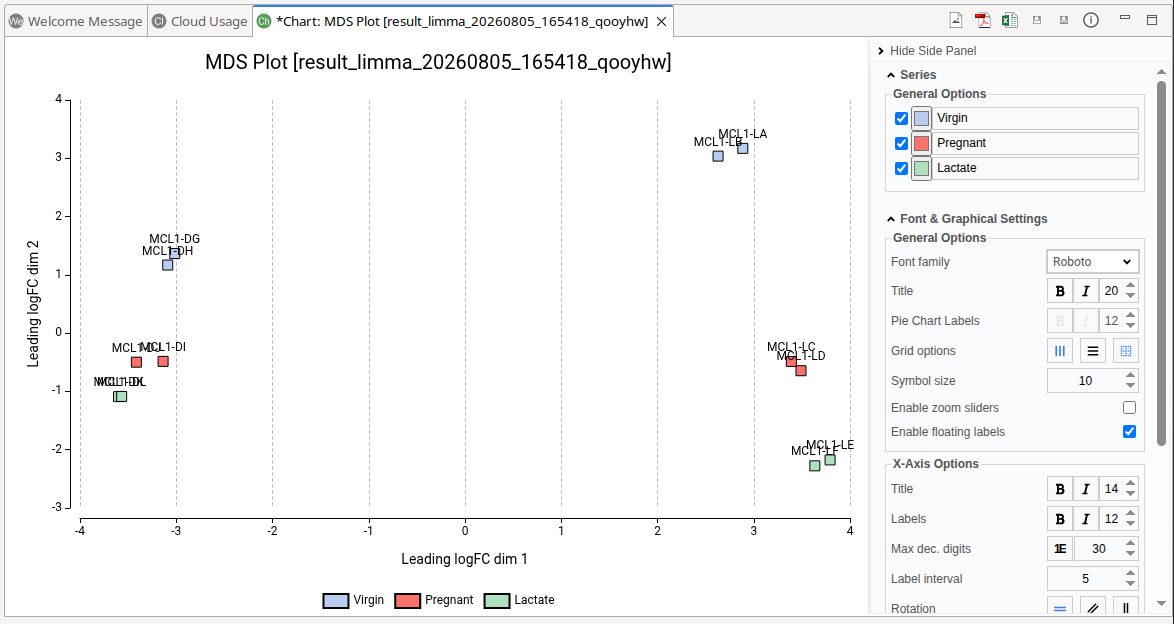
Figure 14: MDS Plot
Volcano Plot
A scatter plot constructed by plotting the negative log of the adjusted p-value (FDR) on the y-axis versus the log2 fold change on the x-axis. Up-regulated and down-regulated features are shown in green and red, respectively.
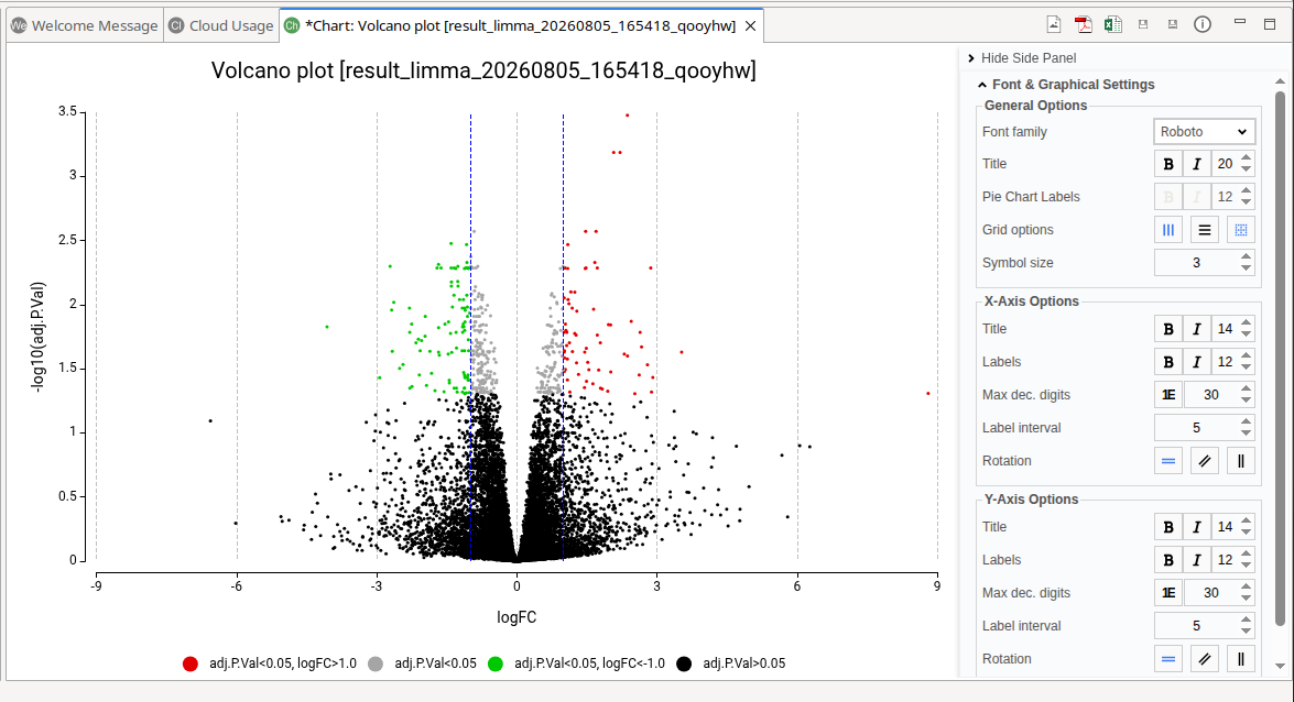
Figure 15: Volcano Plot
Heatmap
A heatmap is a two-dimensional visualization in which numerical values are represented using a color scale. In the context of differential expression analysis, heatmaps are commonly used to visualize the expression patterns of selected features across all samples.
The rows represent features, while the columns represent samples. The color of each cell reflects the expression level of a feature in a given sample, allowing patterns such as co-regulation or sample similarity to be easily identified.
The dendrograms displayed on the left (features) and top (samples) are generated using hierarchical clustering based on the Euclidean distance between expression profiles. This clustering groups together features with similar patterns and samples with similar profiles.
The heatmap supports interactive zooming. It is possible to zoom into a specific cluster by clicking and holding a node in either dendrogram.
The bars shown above the heatmap represent the experimental design factors, illustrating how each sample is associated with the experimental covariates (e.g., condition, treatment, batch).
The features to be displayed can be selected in the wizard via the Select Features parameter:
- Top 50 differentially expressed features, ranked by FDR.
- All differentially expressed features.
- Custom feature list, provided as a list of feature IDs.
Note: Differentially expressed features are those labeled as UP or DOWN in the project table (column Tags). The thresholds used to classify features as up- or down-regulated can be adjusted using the option Set Up/Down Tags.
The wizard also allows defining the expression values used for visualization with the Expression Data parameter, which can be the raw input values or the counts-per-million equivalent, with additional transformations available:
- Logarithm: Reduces the dynamic range of the data, making differences among moderately expressed features more visible and reducing the dominance of highly expressed ones.
- Z-score: Standardizes the values for each feature across samples by centering the mean to zero and scaling by the standard deviation. This highlights relative changes between samples rather than absolute levels, making it easier to identify clusters of features with similar patterns.
These transformations are applied only for visualization purposes and do not affect the statistical results of the differential expression analysis.
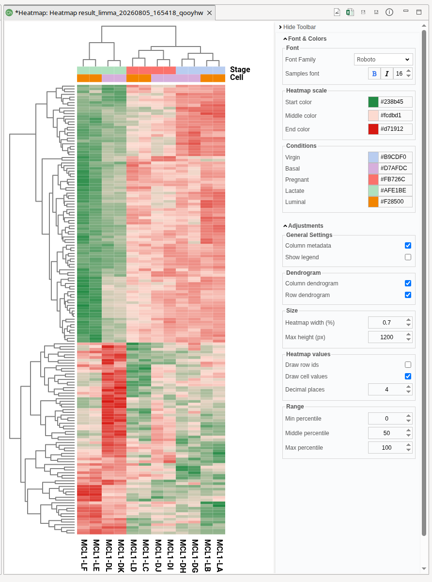
Figure 16: Heatmap
Export
Besides the generic Export Table, this object contains the following export options.
Export Raw Counts
Export the raw input values (counts or intensities, depending on the Input Data Type) to a text file. It does not contain the features discarded during the filtering step.
Export Experimental Design
Export the experimental design to a tab-separated file. The first column contains the samples, whereas the rest are the experimental factors.
Export Ranked List
Export a Ranked List with features in one column and the rank in another column. Rank value for each feature is computed using the following formula: Rank = sign(logFC) * -log10(P-Value)
Context Menu
Besides the generic context menu options, the available action for this object is:
- Extract Selection to New Tab: Extract the data from the selected rows and open it in a new tab.